Backpropagation From Scratch

Most explanations of backprop either wave their hands at the chain rule or bury you in index notation. This post is the version I wish I'd had: a compact shorthand for tracing gradients through any feedforward network, plus the exact equation-to-code mapping for a small 2-layer network trained on XOR.

The core idea: backprop is just the chain rule, applied one layer at a time, where each stop reuses the work from the stop before it. Once that clicks, the "scary" 5-term products stop being scary — they're just a few 2-term multiplications chained together.

---

The network

x → z1 = xW1 + b1 → a1 = ReLU(z1) → z2 = a1W2 + b2 → ŷ = σ(z2) → L = BCE(ŷ, y)

• x: input, shape (m, 2) — m samples, 2 features

• W1: (2, H), b1: (1, H) — first linear layer, H hidden units

• W2: (H, 1), b2: (1, 1) — second linear layer

• Hidden activation: ReLU

• Output activation: sigmoid

• Loss: binary cross-entropy (BCE)

Here's the whole thing laid out visually — forward pass on top, backward pass underneath, dashed lines showing which cached forward value each backward gradient depends on:

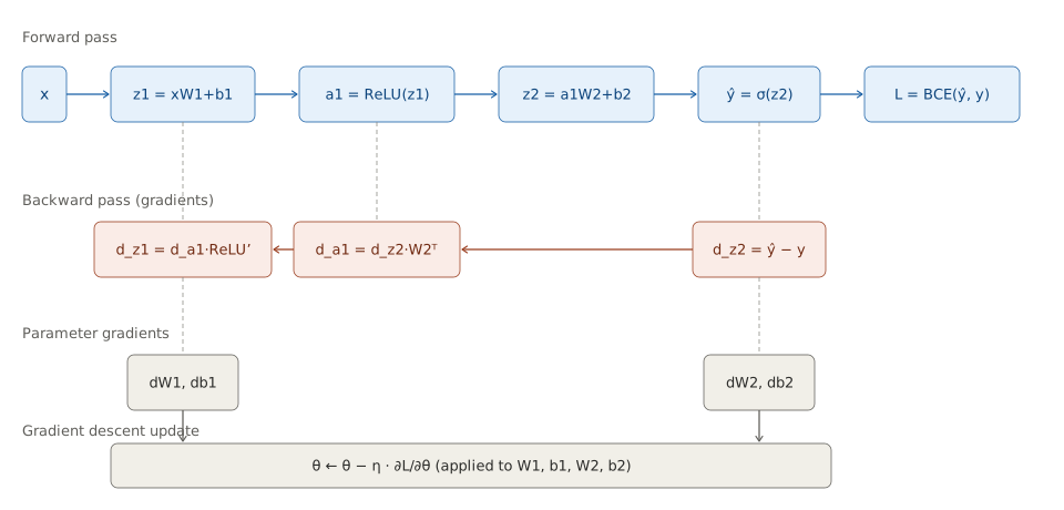
Boxes show x, z1, a1, z2, yhat, L for the forward pass; d_z2, d_a1, d_z1 for the backward pass; dW1/db1 and dW2/db2 for parameter gradients; and the final gradient descent update rule.Forward passBackward pass (gradients)Parameter gradientsGradient descent updatexz1 = xW1+b1a1 = ReLU(z1)z2 = a1W2+b2ŷ = σ(z2)L = BCE(ŷ, y)d_z2 = ŷ − yd_a1 = d_z2·W2ᵀd_z1 = d_a1·ReLU’dW2, db2dW1, db1θ ← θ − η · ∂L/∂θ (applied to W1, b1, W2, b2)

Blue = forward pass. Coral = backward pass gradients. Gray = parameter gradients and the update rule. Dashed gray lines mark which cached forward value each backward step reuses.

---

The one-line shorthand

This is the compressed way to write the whole gradient of W1, term by term:

dLoss/dW1 = (dLoss/dŷ · dŷ/dz2) => dz2
           . dz2/da1              => W2
           . da1/dz1               (activation derivative)
           . dz1/dW1               => x

Read it as: "collapse the loss + output-activation into one named error term, then chain one local derivative per layer going backward."

Everything below is this same idea, spelled out formally and then matched to code.

---

Step 0 — The general principle

For a chain of dependencies w → v → u → L, the chain rule says:

$$\frac{\partial L}{\partial w} = \frac{\partial L}{\partial u}\cdot\frac{\partial u}{\partial v}\cdot\frac{\partial v}{\partial w}$$

Each factor is a local derivative — "how does the next thing downstream change, given a small nudge to the thing upstream." You never skip a link in the chain; however many hops separate L from the variable you're differentiating, that's how many factors you multiply.

The reason backprop doesn't feel like writing one giant product, though, is that several of those factors get reused across different targets (e.g. ∂L/∂z2 is needed for both dW2 and for continuing backward to da1). So instead of re-deriving the full chain for every parameter, you compute a running gradient once per layer, cache it, and reuse it. That's the entire "trick" of backpropagation.

---

Step 1 — Collapse the output layer

$$\frac{\partial L}{\partial z_2} = \underbrace{\frac{\partial L}{\partial \hat y}}{\text{loss derivative}} \cdot \underbrace{\frac{\partial \hat y}{\partial z_2}}{\text{sigmoid derivative}}$$

For BCE loss:

$$\frac{\partial L}{\partial \hat y} = -\frac{y}{\hat y} + \frac{1-y}{1-\hat y}$$

For sigmoid:

$$\frac{\partial \hat y}{\partial z_2} = \hat y(1-\hat y)$$

Multiply them and the messy terms cancel (this is a genuine special-case coincidence of the sigmoid+BCE pairing, not a general law):

$$\frac{\partial L}{\partial z_2} = \hat y - y$$

⚠️ This cancellation is NOT universal. It happens because BCE and sigmoid are a matched pair (same is true for softmax + categorical cross-entropy). Swap in a different loss or output activation — e.g. MSE with a linear output — and you get a different formula (2(ŷ - y), in that case). Always derive both factors separately first; the clean form is a bonus, not a shortcut to memorize blindly.

Code:

d_z2 = self.y_hat - y.float().reshape(-1, 1)   # (m, 1)

---

Step 2 — Gradients for W2, b2

Linear layer: z2 = a1 @ W2 + b2. The local derivatives are:

$$\frac{\partial z_2}{\partial W_2} = a_1^T \qquad \frac{\partial z_2}{\partial b_2} = 1$$

Why a1 shows up for the weight but not the bias: a weight gradient is always (what flowed into this weight) × (how wrong the output was) — nudging a weight only matters in proportion to the input it was scaling. A bias has no such input attached (b2 is just added), so its local derivative is simply 1.

Why we still sum over samples for the bias: b2 is shared — the same number is added into every sample's forward pass. So even though each individual local derivative is 1, b2 influenced the loss through m separate paths (one per sample), and the chain rule for a variable with multiple paths says sum the contribution from every path:

$$\frac{\partial L}{\partial b_2} = \sum_{i=1}^{m} \frac{\partial L}{\partial z_2^{(i)}} \cdot 1$$

$$\frac{\partial L}{\partial W_2} = \frac{1}{m} a_1^T \cdot (\hat y - y) \qquad \frac{\partial L}{\partial b_2} = \frac{1}{m}\sum_{i=1}^m (\hat y_i - y_i)$$

(The 1/m is separate from the chain rule — it's there because the loss itself is averaged over the batch: L = (1/m) Σ L_i, so every gradient inherits that same averaging factor.)

Code:

self.dw2 = (self.a1.T @ d_z2) / m               # (H, 1) — matches W2's shape
self.db2 = torch.sum(d_z2, dim=0, keepdim=True) / m   # (1, 1) — matches b2's shape

Shape check: a1.T is (H, m), d_z2 is (m, 1) → matmul contracts over m (summing across samples automatically) → (H, 1). The matmul is the "sum over paths" — for weights, matrix multiplication does the summing implicitly; for the bias, there's no second axis for @ to contract against, so the sum has to be written explicitly.

---

Step 3 — Propagate the error back to the hidden layer

This step has two separate questions bundled into it, and it helps to keep them apart.

3a. "How much blame does each hidden unit share?" → da1

$$\frac{\partial L}{\partial a_1} = \frac{\partial L}{\partial z_2}\cdot\frac{\partial z_2}{\partial a_1} = (\hat y - y)\cdot W_2$$

Since z2 = a1 @ W2 + b2 is linear in a1, ∂z2/∂a1 = W2 — same "derivative of cx is c" rule as before, just isolating the other variable this time.

Intuition: the output had one shared error signal. Each hidden unit gets blamed in proportion to how strongly it was connected to the output via its weight in W2. A unit with a large weight had more say in the final answer, so it gets a bigger share of the blame.

Code:

d_a1 = d_z2 @ self.w2.T    # (m,1) @ (1,H) -> (m, H)

3b. "Was this unit even switched on?" → dz1

$$\frac{\partial L}{\partial z_1} = \frac{\partial L}{\partial a_1}\cdot\frac{\partial a_1}{\partial z_1}$$

ReLU's local derivative is a gate:

$$\frac{\partial a_1}{\partial z_1} = \begin{cases}1 & z_1 > 0 \text{ (unit active, pass-through)}\0 & z_1 \le 0 \text{ (unit off, blocked)}\end{cases}$$

Intuition: Step 3a assigns blame based on the weights, regardless of whether the unit actually fired. Step 3b corrects that — if a unit was inactive (clipped to zero by ReLU), nudging its pre-activation slightly wouldn't have changed the forward pass at all, so it can't be credited or blamed for the current error, no matter what Step 3a assigned it.

This is the exact mechanism behind "dead ReLU": if a unit's z1 is negative for every sample in the dataset, this mask is 0 everywhere for that unit → its weight gradients are permanently zero → it can never recover. (Leaky ReLU fixes this by using a small nonzero slope, e.g. 0.01, instead of a hard 0, keeping the gate slightly open.)

Code:

self.dz1 = d_a1 * (self.z1 > 0).float()   # (m, H)

---

Step 4 — Gradients for W1, b1

Exactly the same pattern as Step 2, one layer earlier. z1 = x @ W1 + b1:

$$\frac{\partial L}{\partial W_1} = \frac{1}{m} x^T \cdot \frac{\partial L}{\partial z_1} \qquad \frac{\partial L}{\partial b_1} = \frac{1}{m}\sum_{i=1}^m \left(\frac{\partial L}{\partial z_1}\right)_i$$

Code:

self.dw1 = (x.T @ self.dz1) / m                        # (2, H) — matches W1
self.db1 = torch.sum(self.dz1, dim=0, keepdim=True) / m # (1, H) — matches b1

---

Step 5 — Update the weights

$$\theta \leftarrow \theta - \eta,\frac{\partial L}{\partial \theta}$$

for every parameter θ (W1, b1, W2, b2). This is plain gradient descent — subtract because the gradient points toward steepest increase, so subtracting it moves you downhill.

self.w1 -= learning_rate * self.dw1
self.b1 -= learning_rate * self.db1
self.w2 -= learning_rate * self.dw2
self.b2 -= learning_rate * self.db2

---

The full chain for W1, all five terms in one place

$$\frac{\partial L}{\partial W_1} = \underbrace{\frac{\partial L}{\partial \hat y}}{1}\cdot\underbrace{\frac{\partial \hat y}{\partial z_2}}{2}\cdot\underbrace{\frac{\partial z_2}{\partial a_1}}{3}\cdot\underbrace{\frac{\partial a_1}{\partial z_1}}{4}\cdot\underbrace{\frac{\partial z_1}{\partial W_1}}_{5}$$

Grouped exactly the way the code builds it up, left to right:

Cached variable	Terms it represents	Code
d_z2	terms 1 × 2	y_hat - y
d_a1	terms 1,2 × 3	d_z2 @ W2.T
d_z1	terms 1,2,3 × 4	d_a1 * (z1>0)
dW1	terms 1,2,3,4 × 5	x.T @ d_z1

Each named variable is a running partial product — "all terms multiplied so far, stopped at this point in the chain." You never write the full 5-term product directly; you build it incrementally, and each stopping point is reused (d_z2 for both dW2 and continuing to d_a1; that reuse is why it's called "back-propagation."

---

Generalizing beyond this network

Two things change if you swap architectures — everything else in this shorthand stays fixed.

1. The activation's local derivative (step 3b's factor) — swap in whatever activation you're using:

Activation	Local derivative
ReLU	1 if z>0 else 0
Leaky ReLU	1 if z>0 else 0.01
Sigmoid	a(1-a) (using the output, a)
Tanh	1 - a²

2. The loss/output-activation collapse (step 1) — the ŷ - y shortcut only applies to the sigmoid+BCE (or softmax+categorical-cross-entropy) pairing. For any other pairing (e.g. linear output + MSE), redo the two-factor multiplication explicitly rather than assuming it simplifies the same way.

Everything else — the linear-layer rules (dW = input.T @ upstream, db = sum(upstream), d_input = upstream @ W.T) — is fixed machinery that never changes, no matter the activation, loss, or network depth.

The reusable checklist, for any network:

1. Collapse the output: ∂L/∂ŷ · ∂ŷ/∂z_last → name it d_z_last

2. For each layer going backward, repeat:

   • d_a[layer] = d_z[layer+1] @ W[layer+1].T (redistribute blame through weights)

   • d_z[layer] = d_a[layer] * activation'(z[layer]) (gate by whether the unit was active)

3. At each linear layer, before moving further back:

   • dW[layer] = input_to_layer.T @ d_z[layer]

   • db[layer] = sum(d_z[layer], over batch)

That's the whole thing, for any depth, any activation, any loss — swap in the right local derivative in steps 1 and 2, everything else is the same pattern.

---

Full code

Here's the complete, corrected class — bias terms included, ReLU forward and backward pass kept consistent, no double-activation bugs. This is what all the snippets above assemble into.

import torch

class FeedForwardNetwork:
    def __init__(self):
        HIDDEN_SIZE = 4
        INPUT_SIZE = 2
        OUTPUT_SIZE = 1

        # He/Kaiming-style scaling keeps ReLU pre-activations in a reasonable
        # range at init, which matters a lot for a network this small — see
        # the "dead ReLU" note below.
        self.w1 = torch.randn(INPUT_SIZE, HIDDEN_SIZE) * (2.0 / INPUT_SIZE) ** 0.5
        self.w2 = torch.randn(HIDDEN_SIZE, OUTPUT_SIZE) * (2.0 / HIDDEN_SIZE) ** 0.5
        self.b1 = torch.zeros(1, HIDDEN_SIZE)
        self.b2 = torch.zeros(1, OUTPUT_SIZE)

    def forward(self, x):
        # Hidden layer
        self.z1 = x @ self.w1 + self.b1
        self.a1 = torch.relu(self.z1)

        # Output layer
        self.z2 = self.a1 @ self.w2 + self.b2
        self.y_hat = torch.sigmoid(self.z2)
        return self.y_hat

    def backward(self, x, y):
        m = x.shape[0]

        # Step 1: collapse loss + output activation -> error at z2
        d_z2 = self.y_hat - y.float().reshape(-1, 1)

        # Step 2: gradients for W2, b2
        self.dw2 = (self.a1.T @ d_z2) / m
        self.db2 = torch.sum(d_z2, dim=0, keepdim=True) / m

        # Step 3: propagate error back to the hidden layer
        d_a1 = d_z2 @ self.w2.T                     # redistribute blame through W2
        d_z1 = d_a1 * (self.z1 > 0).float()          # gate by whether ReLU fired

        # Step 4: gradients for W1, b1
        self.dw1 = (x.T @ d_z1) / m
        self.db1 = torch.sum(d_z1, dim=0, keepdim=True) / m

    def update_weights(self, learning_rate):
        self.w1 -= learning_rate * self.dw1
        self.b1 -= learning_rate * self.db1
        self.w2 -= learning_rate * self.dw2
        self.b2 -= learning_rate * self.db2

Training loop, on XOR:

torch.manual_seed(0)
ffn = FeedForwardNetwork()

X = torch.tensor([[0, 0], [0, 1], [1, 0], [1, 1]], dtype=torch.float)
Y = torch.tensor([0, 1, 1, 0], dtype=torch.float)

learning_rate = 0.05
epochs = 50000

for epoch in range(epochs):
    y_hat = ffn.forward(X)
    ffn.backward(X, Y)
    ffn.update_weights(learning_rate)

    if (epoch + 1) % 5000 == 0:
        loss = torch.nn.functional.binary_cross_entropy(y_hat, Y.reshape(-1, 1))
        print(f"Epoch [{epoch+1}/{epochs}], Loss: {loss.item():.4f}")

# Check predictions — forward() already applies sigmoid, don't apply it twice
with torch.no_grad():
    for i in range(X.shape[0]):
        pred = ffn.forward(X[i:i+1]).item()
        print(f"Input: {X[i].tolist()} -> Predicted: {pred:.4f}, Expected: {Y[i].item()}")

Two bugs worth knowing about, because they're easy to reproduce:

• Dead ReLU. With unscaled torch.randn initialization, it's easy for a hidden unit's pre-activation to be negative across every training sample from the start — the ReLU gate (z1 > 0) then stays 0 forever for that unit, so it never updates. The He-scaled init above (* (2.0 / fan_in) ** 0.5) makes this far less likely, though not impossible — if training plateaus, try a different seed.

• Double sigmoid. forward() already returns a sigmoid-activated value, so calling torch.sigmoid() again on its output squashes an already-squashed number and compresses everything toward the middle of the range. If your predictions all look suspiciously close to 0.5 or 0.73, check for this first.